OPTIMIZE OUR LIDAR ODOM

 

[STEP 1: NORMALIZE THE ERROR

 

FUNCTION]

 

Jack Mo (mobangjack@whu.edu.cn)

http://twogen.cn

QUICK REVIEW

In the last chapter, we discussed a straight method to use lidar as an odometer, and implemented it with a piece of c++ code. The test showed that our implementation did work, though not so fine as expected. This chapter we will review the leak of our method and try to improve the performance.

CORE METHOD

For a measurement of a limit space in time t, we have a vector . For another measurement of the same space in time t+1, we have another vector . Note that we suppose the two neighboring measurements in time sequence always happen in the same space. So one of the measurement result can be considered as the rotation-translation transform of the other, which can be represented by the following formula.

(1)

There we try to measure the distance between the two neighboring measurements using the error function. Notice that this is actually operated in the rectangular coordinate. To avoid introducing more symbols, we just write as below.

(2)

By combining eq(3) and eq(4) which we’ve derived before, we finally have an numerical form of error function as eq(5). There we play a small trick. We perform rotation transformation by circulating the vector x instead of using eq(1) directly. That’s the goodness to vectorize the lidar measurenment result. You may have noticed it in our c++ code.

(3)

(4)

(5)

By minimizing eq(5), we get the nearest distance (or the minimum error) between and , and the coordinate arg and .

(6)

Then we go back to eq(3) and eq(4) to retrieve the tangiable coordinate rotation-translation parameters and . By using this method iteratively, we have the complete rotation and translation parameters at time t.

(7)

(8)

NORMALIZE THE ERROR FUNCTION

The target we’re trying to optimize is eq(5). Let’s think about it a little more. First let’s have a look of the visualization of lidar measurements.

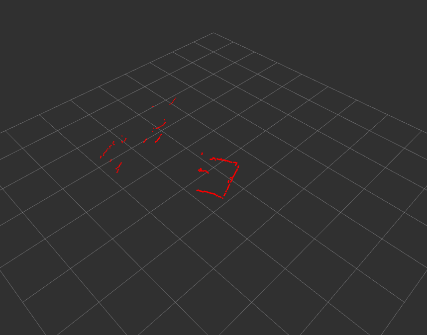
Graph 1. Visualization of LIDAR Measurenments

As the picture shown above, the range of lidar is very limited. Meanwhile, there are points come and go as the lidar pose changes. Thus the number of valid range data we get each time may be variant. Now the problem is obvious.The error function we use is actually sum of square error. In this condition, the computation of and may not be in the same space. We need to normalize the error function to solve this problem. That is, we should use mean sqaure error instead of sum of square error, which is corrected as below.

(9)

The formula above makes and comparable. This seems to have nothing to do with the robustness or accuracy of our current lidar odometry, because it won’t change the result of eq(6), but is vital when it comes to choose the best matched mesurement among generations. We will discuss this later in the following chapters.